Quad Bayer in the Frequency Domain – Part 1: Spectrum Analysis
I also plan a Part 2: Using Spectral Redundancies, which will look at how to actually exploit the redundancies discussed in this first part.
Apparently, Quad Bayer image sensors have existed since 2014. But I only learned about Quad Bayer (also called Tetracell, 4-cell, Quadra, Quad Pixel, Quad CFA) recently and the following statement got me interested: “De-Bayering Bayer data […] is a technology […] that has been developed for now 25 years. de-Bayering Quadra is a completely different beast. It is way more complicated than one may think.” (32:20).
I worked on de-Bayering myself many years ago and specifically used insights from spectral analysis of the Color Filter Array (CFA) signal. A quick search did not bring up any discussion of spectral properties of the Quad Bayer pattern (Let me know what I may have missed!). I plotted the spectrum of an example image – and I wanted to know more. 🤓
Images in the Frequency Domain
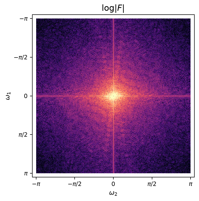
The spectrum of an ordinary image looks like the above. This is the spectrum of the average of R, G, and B but each component by itself looks very similar. There is a lot of energy at low frequencies (shown at the center). The energy falls off quickly towards the edges of the spectrum. The edges of the spectrum at $\pm\pi$ are the maximum frequencies that can be represented by the discrete pixel grid.
A. Classic Bayer
Bayer CFA in the Frequency Domain
A Bayer CFA image $f_\text{CFA}$ is a pointwise mixture of the $RGB$ color channels $f_c$ at pixel position $\mathbf{n} = (n_1, n_2)$,
$$f_\text{CFA}[\mathbf{n}] = \sum_{c \in \{R,G,B\}} f_c[\mathbf{n}]\, m_c[\mathbf{n}]$$where $m_c[\mathbf{n}] \in \{0,1\}$ is the indicator for color $c$. For example, $m_R[\mathbf{n}]$ is 1 for all red pixel positions $\mathbf{n}$, and it is 0 otherwise; $m_G[\mathbf{n}]$ is 1 for all green pixel positions…
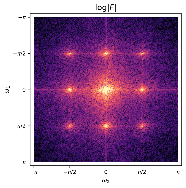
When viewing the spectrum of the CFA of an example image, we observe a few interesting spectra in the corners and the border
which are not immediately obvious from the above formula:
20 years ago, Eric Dubois showed that $f_\text{CFA}$ can be re-written as
$$\begin{split}f_\text{CFA}[\mathbf{n}] &= L[\mathbf{n}] \\ \, &- C_1[\mathbf{n}]\,(-1)^{n_1+n_2}\\ \, &+ C_2[\mathbf{n}]\bigl((-1)^{n_1} - (-1)^{n_2}\bigr) \end{split}$$consisting of three spectral components that are modulated by carriers at different 2D frequencies:
| Component | Carrier(s) | Amplitude |
|---|---|---|
| $L = \tfrac{1}{4}(R + 2G + B)$ | $(0, 0)$ | $1$ |
| $C_1 = \tfrac{1}{4}(R - 2G + B)$ | $(\pm\pi, \pm\pi)$ | $1$ |
| $C_2 = \tfrac{1}{4}(R - B)$ | $(\pm\pi, 0),\; (0, \pm\pi)$ | $1$ |
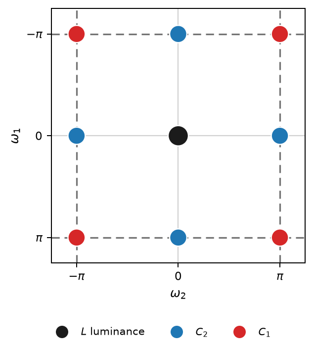 The luminance component, $L$, at the center of the spectrum is just the average of the CFA’s GRBG pattern.
In addition, there are two chrominance components, $C_1$ and $C_2$, with their carriers exactly on the Nyquist boundary:
$C_1$ in the diagonal corners and $C_2$ on the horizontal and vertical edges of the spectrum.
The luminance component, $L$, at the center of the spectrum is just the average of the CFA’s GRBG pattern.
In addition, there are two chrominance components, $C_1$ and $C_2$, with their carriers exactly on the Nyquist boundary:
$C_1$ in the diagonal corners and $C_2$ on the horizontal and vertical edges of the spectrum.
Redundancy of $C_2$
The factor $((-1)^{n_1} - (-1)^{n_2})$ places the same $C_2$ at two separate carrier locations: the horizontal Nyquist edge $(\pi, 0)$ and the vertical edge $(0, \pi)$. These are two independent observations of $C_2$: the copy at $(\pi, 0)$, $C_{2,h}$, may be contaminated by luminance energy concentrated along horizontal frequencies, while the copy at $(0, \pi)$, $C_{2,v}$, may be contaminated by vertical luminance energy. In a natural image, one of the two is usually cleaner.
Dubois exploits this by forming an adaptive estimate
$$\hat{C}_2 = w\,\hat{C}_{2,h} + (1-w)\,\hat{C}_{2,v}$$where $w$ is determined locally by the estimated horizontal and vertical luminance energy.
$C_1$ has only a single carrier at the Nyquist corner, so there is no second copy to adapt with.
$L$ from subtracting –not filtering out– the chrominances
In Dubois’s approach, $C_1$, $C_{2,h}$, $C_{2,v}$ are extracted using bandpass filters. But the luminance is not recovered by low-passing the mosaicked signal. Instead, the modulated chrominance estimates are subtracted:
$$\begin{split}\hat{L}[\mathbf{n}] &= f_\text{CFA}[\mathbf{n}] \\ \, &- \hat{C}_2[\mathbf{n}]\bigl((-1)^{n_1} - (-1)^{n_2}\bigr) \\ \, &+ \hat{C}_1[\mathbf{n}]\,(-1)^{n_1+n_2}\end{split}$$The benefit of this approach is that any improvement in the chrominance estimates directly improves the luminance estimate. This applies especially to the adaptive estimate of $C_{2}$. It also allowed significant improvements from additionally applying restoration filtering to the LCC components.
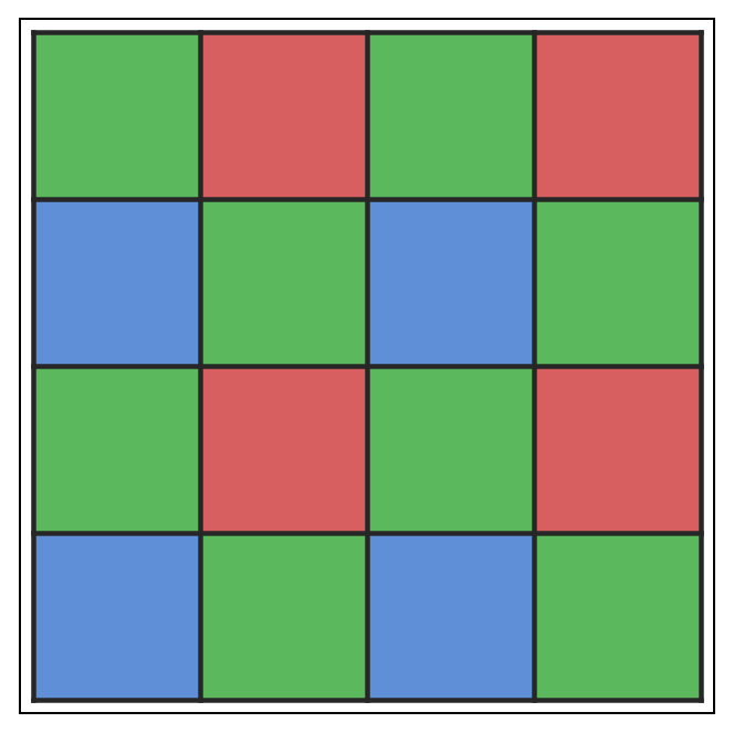
B. The Quad Bayer Pattern
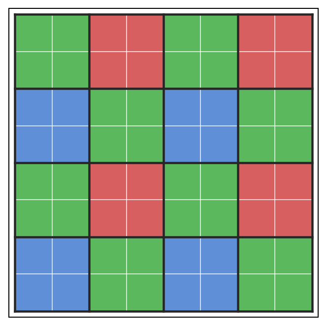
Quad Bayer compared to Bayer
In some sense, Quad Bayer is much harder: Quad Bayer widens each color filter cell to cover $2\times2$ pixels, retaining only half the CFA resolution. Thus the carriers migrate inward to $\pi \rightarrow \pi/2$. Chrominance spectra move from the Nyquist edge to the mid-band – much closer to the luminance band with much higher chance of interfering with it.
From a different angle, Quad Bayer provides a new opportunities: Quad Bayer doubles pixel resolution for each color of the Bayer pattern, we get a $2\times2$ block of pixels instead of one. The available spectrum widens and Nyquist boundaries move away from the modulated chrominance spectra – giving much more room for chrominances, as well as for the luminance.
The Frequency Domain Formulation
Whichever way you view it, the Quad Bayer modulation formula becomes
$$\begin{split}f_\text{CFA}[\mathbf{n}] &= L[\mathbf{n}] \\ \, &- C_1[\mathbf{n}]\,s[n_1]\,s[n_2] \\ \, &+ C_2[\mathbf{n}]\bigl(s[n_1] - s[n_2]\bigr)\end{split}$$using the same $L$/$C_1$/$C_2$ definitions as above and where
$$s[n] = (-1)^{\lfloor n/2\rfloor} = \cos\!\tfrac{\pi n}{2} + \sin\!\tfrac{\pi n}{2}$$is a period-4 square wave ($+1,+1,-1,-1$).
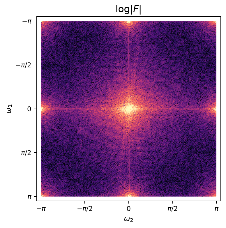
The carriers are now at half the frequency:
| Component | Carrier(s) | Amplitude |
|---|---|---|
| $L$ | $(0, 0)$ | $1$ |
| $C_1$ | $(\pm\tfrac{\pi}{2}, \pm\tfrac{\pi}{2})$ | $1/2$ |
| $C_2$ | $(\pm\tfrac{\pi}{2}, 0),\; (0, \pm\tfrac{\pi}{2})$ | $1/\sqrt{2}$ |
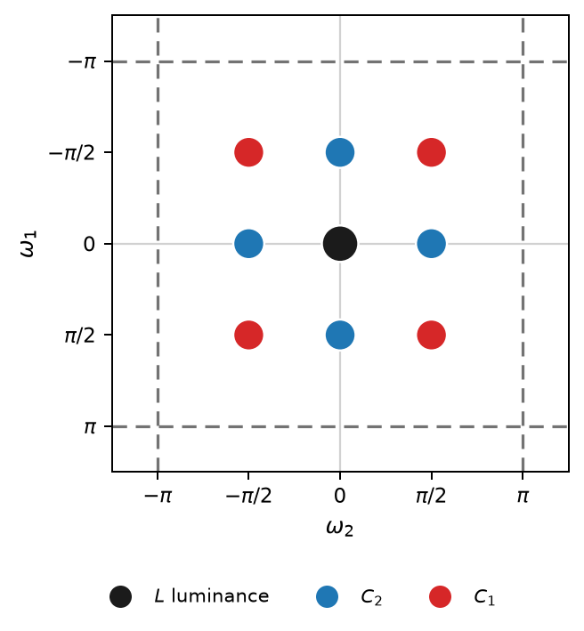
The chrominance amplitudes are smaller. As noted above, $s[n]=\cos\tfrac{\pi n}{2}+\sin\tfrac{\pi n}{2}$. Unlike Bayer’s $\cos(\pi n)$, this is an interior frequency, so its two conjugate carriers stay distinct rather than recombining at the Nyquist boundary. For $C_2$ the cosine and sine halves meet at the same carrier in quadrature, giving $\sqrt{(1/2)^2+(1/2)^2}=1/\sqrt2$; for $C_1$ the product $s[n_1]s[n_2]$ splits into two unit sinusoids at separate diagonal carriers, each contributing $1/2$.
Quad Bayer Redundancies
While the normalized spectral distance between spectra is much narrower, there are still three types of redundancy that may be useful for de-Bayering.
1. Preserved $C_2$ redundancy
The term $s[n_1] - s[n_2]$ still places $C_2$ at two independent carriers, now $(\pi/2, 0)$ and $(0, \pi/2)$. Dubois’s adaptive $H/V$ blending as mentioned above can in principle be applied to Quad Bayer, too.
2. Additional $C_1$ redundancy
The reason $C_1$ can split in Quad Bayer but not in Bayer lies in carrier position: in Bayer, the $C_1$ carrier is at the Nyquist corner $(\pi, \pi)$. In two dimensions, the frequencies $(\pi, \pi)$ and $(\pi, -\pi)$ are the same point modulo $2\pi$. Thus the two diagonals coincide, and only one real modulation exists. In Quad Bayer, the carrier moves to $(\pi/2, \pi/2)$, which is distinct from $(\pi/2, -\pi/2)$. Expanding $s[n_1] s[n_2]$:
$$s[n_1]\,s[n_2] = \cos\!\bigl(\tfrac{\pi}{2}(n_1 - n_2)\bigr) + \sin\!\bigl(\tfrac{\pi}{2}(n_1 + n_2)\bigr),$$we observe that $C_1$ now splits into two independent diagonal carriers:
- the anti-diagonal cosine at $(\pi/2, -\pi/2)$ and
- the main-diagonal sine at $(\pi/2, \pi/2)$.
Each is an independent copy and affected differently by diagonal-frequency luminance content, providing a main-/anti-diagonal redundancy. This can be exploited in an analogous manner to that of $C_2$ for horizontal and vertical frequencies.
3. Sideband symmetry
Because $C_1$ and $C_2$ each are real signals, their respective spectra satisfy $C(-\boldsymbol{\nu}) = C^*(\boldsymbol{\nu})$. Therefore, each modulated copy is Hermitian about its carrier $\boldsymbol{\omega}_0$: the spectrum at $\boldsymbol{\omega}_0 + \boldsymbol{\nu}$ is the conjugate of the value at $\boldsymbol{\omega}_0 - \boldsymbol{\nu}$. One half-plane through the carrier suffices for exact recovery. In 2D, the dividing diameter can take any orientation — a free continuous parameter — and different orientations expose different parts of the luminance background, so the half-plane can be chosen to minimize crosstalk from other bands.
This symmetry may also help differentiate the signal from the generally asymmetric crosstalk of other bands.
This sideband redundancy is within-carrier and in addition to the independent copies of $C_1$ and $C_2$. In Quad Bayer, both apply simultaneously. If and how this may be exploited in practice is the subject of Part 2.
Disclaimer
No FFTs are used in the application of these methods. It may be worth mentioning that the frequency-domain framework here is purely analytical: it motivates why certain operations and adaptive strategies work, but no FFT appears in the demosaicking algorithms themselves, their optimization, or even the filter design. These are all in the pixel domain. The only use of FFT here has been for the illustrative spectra of real images shown above.
I have not done much research on the state of the art. I tried to make sure that this has not very obviously been done before, but beyond that I just wanted to get going.
Lastly, AI helped. I am not much of a writer and without AI I probably would not have written this. AI summarized prior work, helped sort out and formalize my intuition and mental models, create illustrations, etc.